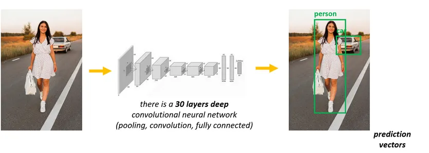
Top Object Detection Techniques in Computer Vision

Object detection: Locating the presence of objects with a
bounding box and types or classes of the located objects in an image
or video is called object detection.

Input: An image with one or more objects. Output: One or more
bounding boxes (e.g. defined by a point, width, and height), and a
class label for each bounding box.

Some of the famous Object detection techniques

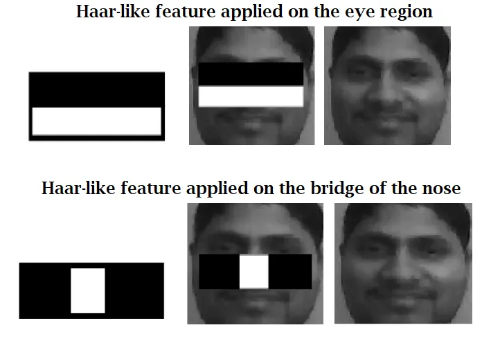
1 .Viola Jones:

This technique was formulated by Paul viola and Micheal Jones in
2001. Although it can be trained to detect a variety of object
classes, It was giving better results on face detection.It uses
Haar-cascade classifiers technique to detect the object without
using Neural Networks.This algorithm tries to find the most relevant
features for a human faces(ex : eyes,nose,lips and forehead).If the
Algorithm does not find the most relevant features it comes to
conclusion that there is no Human face on the region of the image.

Advantages:

Detection is very fast
Simple to understand and implement
Less data needed for training than other ML models
No resizing of images needed (like with CNN’s)

Disadvantages:

Training time is very slow
Restricted to binary classification
Mostly effective when face is in frontal view
May be sensitive to very high/low exposure (brightness)
High true detection rate, but also high false detection rate

Applications:

Attendance recording for employees based on face detection instead
of fingerprint.

2 .HOG(Histogram of oriented Gradients)

This approach was first published by navneet Dadal and Bill Triggs
in 2005 this approach out performed on face detection and Object
detection etc. this approach uses gradients: Difference in pixel
intensities for pixel’s right next to each other(surrounding
pixels).Using grayscale images and using blurring (gaussian
smoothing) have a negative effect on the precision of the final
classification algorithm.

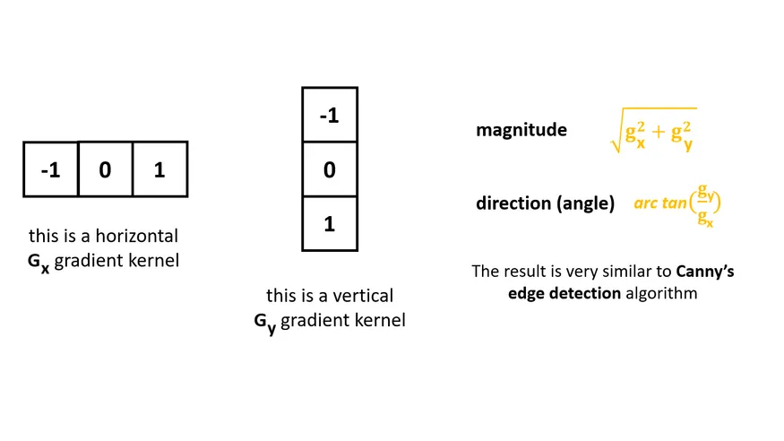
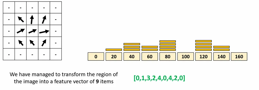
Oriented Gradient means which tells us the direction of greatest
intensity change in the neighborhood of pixel(x,y).

The angles are within the range[0,180]. So called un-signed
gradients. A gradient arrow and the one 180 degrees opposite to it
are considered the same. Finally we have to calculate the histogram
containing 9 bins corresponding to angels in degrees.

Advantages:

Gives better results on face detection if the location of the face even changes.
Easy to detect binary objects in an image.

Disadvantages:

Take lot of time to execute.
Does Not give better results if there are multiple objects.
Applying the sliding window and Normalization data manually is a challenging thing.

Applications:

Pedestrian detection in highways.
Face detection for attendance and mobile lock screens.

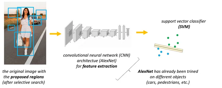
3 .Regional Based Convolutional Neural Networks (R-CNN’s)

This concept was implemented using convolutional neural networks
where it takes an input image and produces a set of bounding boxes
as output and each bounding box contains an object and also the
category.

It is used for object detection: cars , pedestrians,people etc.
The main problem with standard CNN is that we have to consider several regions of the image(that contains no objects at all)

RCNNs can effectively reduce the number of iterations using a
concept called selective search.

This selective search algorithm generates the so-called region
proposals and these regions are fed into a neural network.

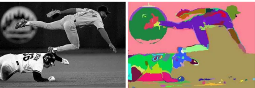
Selective search algorithm uses segmentation: so the algorithm
groups adjacent regions that are similar to each other. We group
pixels into a smaller number of segments.

Selective search algorithm use the result of Felzenszwalb-huttenlocher transform on the actual image.
The initial proposed regions are the segmented parts after the transformation.
The algorithm keeps grouping segments based on similarity(color,texture,size and shape)

After applying selective search the proposed regions will be
selected and sent to the neural network.

So the neural network were already trained on training data and each
region on the image sent to the neural network and generated output
vectors were sent to support vector machine algorithms for finding
the class label.

Problems with R-CNN’s

It still takes a huge amount of time to train the network as you would have to classify 2000 region proposals per image.
It cannot be implemented real time as it takes around 47 seconds for each test image.
The selective search algorithm is a fixed algorithm. Therefore, no learning is happening at that stage. This could lead to the generation of bad candidate region proposals.
Training time is around 84 hrs.

4. Fast R-CNN

This approach is similar to the R-CNN algorithm. But, instead of
feeding the region proposals to the neural network , we feed the
input image to the neural network to generate a convolutional
feature map. From the convolutional feature map, we identify the
region of proposals and warp them into squares and by using a RoI
pooling layer we reshape them into a fixed size so that it can be
fed into a fully connected layer. From the RoI(Region of interest)
feature vector, we use a softmax layer to predict the class of the
proposed region and also the offset values for the bounding box.

The reason Fast R-CNN algorithm is faster than R-CNN is because you
don’t have to feed 2000 region proposals to the convolutional neural
network every time. Instead, the convolution operation is done only
once per image and a feature map is generated from it.

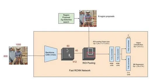
Fast R-CNN drastically improves the training (8.75 hrs vs 84 hrs)
and detection time from R-CNN. It also improves Mean Average
Precision (mAP) marginally as compared to R-CNN.

Problems with R-CNN’s

Most of the time taken by Fast R-CNN during detection is a selective
search region proposal generation algorithm. Hence, it is the
bottleneck of this architecture which was dealt with in Faster
R-CNN.

5. Faster R-CNN

Faster R-CNN uses a region proposal method to create the sets of
regions. It possesses an extra CNN for gaining the regional
proposal, which we call the regional proposal network. In the
training region, the proposal network takes the feature map as input
and outputs region proposals. And these proposals go to the ROI
pooling layer for further procedure.

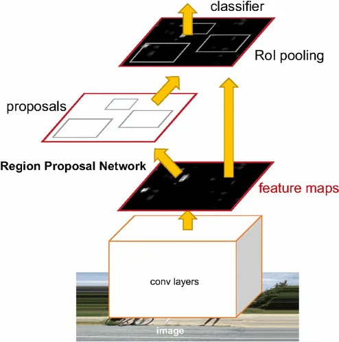
Comparison between Faster R-CNN and Fast R-CNN

Faster R-CNN is much faster than Fast R-CNN and R-CNN because it is used by RPN(Region Proposal Network) for generating anchor boxes (region proposals).
It can be used in real-time object detection.

Applications

Face detection using Neural Networks.
Face Recognition.
Object tracking

6 .Yolo (You Only Look once)

There are several Minor issues with region based neural network
where it is very accurate but not fast and can not be used in
real-time.we have to pre-train several components of the approach
(CNN,SVM,Linear regression model for bounding boxes etc).yolo can
deal with this issues, it was first published back in 2015 by Joseph
Redmon , Ross Girshick etc.using yolo we can train the model with a
single neural network. First yolo divides the image in 19*19 grids
and each grid sent to the neural network for generating 5 vectors
called it positions and number of class labels so within single CNN
layers entire detecting is going to happen and for managing the
multiple objects we can use NON max suppression and Intersection
over union concepts. So when compared to regional based Neural
networks yolo works in a better manner.yolo algorithm where trained
on coco dataset where we are having 80 labels so we can use its
pre-trained weights directly to detect objects out of those 80. If
we want to create custom data also it is possible using yolo just we
need to annotate and train the network.

Advantages and disadvantages of YOLO

YOLO is orders of magnitude faster(45 frames per second) than
other object detection algorithms.
The limitation of the YOLO algorithm is that it struggles with
small objects within the image, for example, it might have
difficulties in detecting a flock of birds. This is due to the
spatial constraints of the algorithm.

Applications

Vehicle detection.
Number Plate detection.
Covid detection

7. SSD(single shot multibox Detector)

The first step is very similar to YOLO algorithm: we have to divide
the original image upto S*S grid cells.
Each grid is
responsible for detecting objects in that region of the image.there
is a problem again: what if there are Multiple objects in the same
region of the image.we can use default boxes – anchor boxes(these
are pre-trained boxers)
The SSD algorithm makes an assumption about the size and
orientations of the default boxes(we can learn about them from the
training dataset).there are patterns for the aspect ratios and sizes
of the bounding boxes.we assign 6 different types of bounding boxes
to every single grid cell.

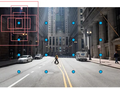
The algorithm will find the bounding box that is the most similar to
the detected object. The advantage of the SSD algorithm is it makes
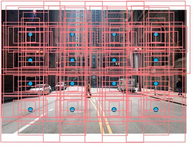
several predictions at different stages of the CNN.

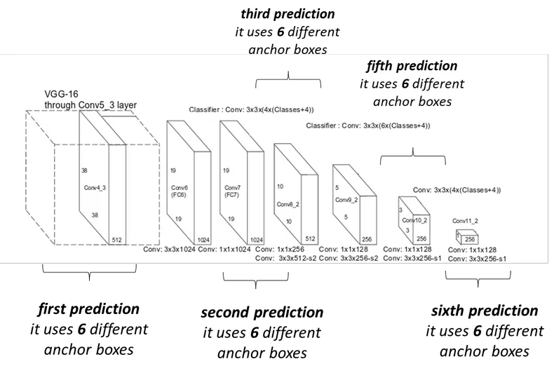
The SSD algorithm makes several predictions at different stages of
the CNN.The feature map is the output of one filter applied to the
previous layer.

The convolutional layers decrease in size progressively and allow
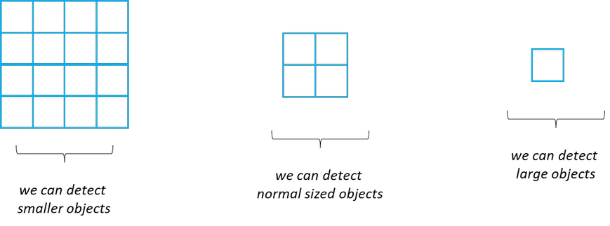
predictions of the detections at multiple scales.

Features at different layers represent sizes of regions in the input
image.The size of the image represented by a feature gets larger and
larger and predictions from the previous layers help in dealing with
smaller objects.

Advantages

Accuracy increases with the number of default boundary boxes at the cost of speed.
Multi-scale feature maps improve the detection of objects at a different scale.